
Pre-trained 3D convolutional neural network for video labelling
The number of videos available on the Internet is growing up rapidly. Every day, each minute, over 400 hours of new videos are uploaded on YouTube.
In this context, an increasing number of experts is trying to analyse these videos for various purposes like search, recommendation, ranking, …
In this post, we will talk about video labelling and Convolutional neural network, a class of deep neural networks, that can be applied to this problem.
Convolutional neural networks
Convolutional neural networks (CNNs), also known as ConvNets, are widely used in computer vision applications, to solve image-classification problems.
Convolution layers look at spatially local patterns by applying the same geometric transformation to different spatial locations (patches) in an input tensor. This idea is applicable to spaces of any dimensionality: 1D (sequences), 2D (images), 3D (volumes) and so on.
In this post we will focus our attention on 3D ConvNets, because they are the best solution for the video labelling problem.
According to Du Tran et al., 3D ConvNet is well-suited for spatiotemporal feature learning. Compared to 2D ConvNet, 3D ConvNet has the ability to model temporal information better, owing to 3D convolution and 3D pooling operations. It is common to use Conv1D layer to process sequences (especially text), the Conv2D layer to process images, and the Conv3D layers to process volumes.
Practical example: Sports1M
To put it as simply as possible, we are going to look at a practical example.
Sports1M is a dataset which contains 1,133,158 video URLs of different sports, that have been annotated with 487 labels.
Since Sports1M is huge, in order to build an efficient neural network, it is necessary an enormous computing power. In fact, in this case, the best solution is a deep neural network with many parameters that have to be estimated (we have ~80 million parameters).
Furthermore, the dataset includes videos available on YouTube, but we have to pay to get the YouTube API key. Fortunately, neural networks for video classification are a subject of active research and pre-trained models on Sports1M are currently available, that can be exploited to extract high-level features to be used in conjunction with other classifiers or by means of Transfer Learning.
In the following, we will use a pre-trained model that is freely-available here. This model was trained using GPU systems that are expensive and difficult to implement.
The code snippets we’ll show are written in Python. You will need the following packages:
- cv2
- matplotlib
- Keras (v. 2.2.4.)
The model must be imported in Python with its weights, and you also need to read the .txt file with the labels.
|
1 2 3 4 5 6 |
model = create_model_sequential() model.load_weights(' /path/to/file/C3D_Sport1M_weights_keras_2.2.4.h5') with open('/path/to/file/labels.txt', 'r') as f: labels = [line.strip() for line in f.readlines()] print('Total labels: {}'.format(len(labels))) |
Since the model has many layers, we won’t display the full structure, but you can see it with the following line of code:
|
1 |
model.summary() |
Note that it is basically a stack of Conv3D and MaxPooling3D layers. The output of every Conv3D and MaxPooling3D is a 4D tensor of shape (frames, height, width, channels).
ConvNet architecture
The convolution operation extracts patches from its input feature map and applies the same transformation to all of these patches, producing an output feature map. This output feature map is still a 4D tensor: it has frames, height, width. Its depth (channels) can be arbitrary, because the output depth is a parameter of the layer, and the different channels in that depth axis stand for filters1 .
Convolutions are defined by two parameters:
- size of patches extracted from the inputs.
- depth of the output feature map: the number of filters computed by the convolution.
Our example started with 64 and ended with 512 filters. For their characteristics, convolution layers learn local patterns instead of global patterns.
Pooling layer
It is common to periodically insert a Pooling layer in-between successive Conv layers in a ConvNet architecture. Its function is to progressively reduce the feature maps to reduce the amount of parameters in the network, and hence to also control overfitting. The Pooling Layer operates independently on every depth slice of the input and resizes it spatially, using the MAX operation. In our network we are using MaxPooling layers with filters of size 2x2x2, except for the first Pooling layer that has a kernel of size 1x2x2. The different structure of the first Pooling layer allows not to merge the temporal signal too early.
Example result
It’s time to test this model. We choose a basketball video available on YouTube link o but you can use another sport video.
First of all, you have to convert the video into a float32 format. You can use the following code.
|
1 2 3 4 5 6 7 8 |
cap = cv2.VideoCapture('/path/to/file/videoplayback.mp4') vid = [] while True: ret, img = cap.read() if not ret: break vid.append(cv2.resize(img, (171, 128))) vid = np.array(vid, dtype=np.float32) |
Our model considers only 16 video frames a time but typically a video is made of a lot of frames. Thus, to assign a label to an entire video, we apply the model to a batch of 16 video frames and, if it assigns a probability higher than 80% to one of the 487 possible labels, we classify the whole video with the given label. If the probability is lower, we switch 100 frames forward. In fact, we assume that frames close to each other are very similar and the probabilities related to the labels won’t change that much.
However, it is possible that none of batches will allow the model to assign a label with a probability higher than 80%.
For this reason we keep track of the frames with the highest probability associated.
|
1 2 3 4 5 6 7 8 9 10 11 12 13 14 15 16 |
import matplotlib.pyplot as plt %matplotlib inline final_output = np.zeros((1, 487)) for frame in range(1, vid.shape[0], 100): X = vid[frame:(frame+16), 8:120, 30:142, :] output = model.predict_on_batch(np.array([X])) if output.max() >= 0.8: final_output = output final_frame = frame break elif output.max() > final_output.max(): final_output = output final_frame = frame plt.plot(final_output[0]) plt.imshow(vid[final_frame]/256) |
In our example case, as it is clear from the following picture, there is a peak of the probability associated with a specific label.

What are the frames that enabled the model to label the video with a high probability? The next figure shows the first frame of the series.

Finally we report code and results.
|
1 2 3 4 5 6 7 8 |
print('Position of maximum probability: {}'.format(output[0].argmax())) print('Maximum probability: {:.5f}'.format(max(output[0]))) print('Corresponding label: {}'.format(labels[output[0].argmax()])) # sort top five predictions from softmax output top_inds = final_output[0].argsort()[::-1][:5] # reverse sort and take five largest items print('\nTop 5 probabilities and labels:') _ =[print('{:.5f} {}'.format(output[0][i], labels[i])) for i in top_inds] |
Position of maximum probability: 367
Maximum probability: 0.91563
Corresponding label: basketball
Top 5 probabilities and labels:
0.91563 basketball
0.07668 streetball
0.00524 wheelchair basketball
0.00072 netball
0.00049 3×3 (basketball)
Test on UCF-101
In order to further assess the performances of our neural network, we need a test set. However, we can’t use Sport1M dataset, because all its videos were used to train the model. We decide to test our model in a slightly different context: action recognition instead of sport recognition.
We use a public dataset, UCF-101 that contains realistic action videos, collected from YouTube, having 101 action categories.
Feature Extraction
Feature extraction consists of using the representations learned by a previous network to extract interesting features from new samples. Then, these features are put as input in a new classifier, which is trained from scratch.
Our model is made of two different parts: the first part is a series of pooling and convolution layers (convolutional base); the second part is a densely connected classifier. We perform feature extraction taking the convolutional base of the model previously trained on Sport1M, giving the new data as input to it and with the output we train a new classifier.
In details, we are giving as input of the neural network a batch of 16 video frames that generate a vector of 4096 elements.
As explained previously, it is possible that frames close to each other are very similar. For this reason, we are considering groups of 16 frames for each video and we switch 50 frames forward to find the next input for our model.
Of course each video can generate more outputs because typically it has more than 66 frames.
After this operation, the output obtained is recorded as two Pandas dataframes on disk, that we will use as train set and as validation. 2
The dataframes have 4096 columns that represent the output features. The train set has 37274 rows and the validation set has 14544 rows corresponding to the number of frames batches analysed.
We train a new classifier on top of this output and in particular, we have tested a Random Forest, a multi-class linear SVM and a new densely connected classifier.
Random Forest and SVM parameters have been estimated using a grid search with cross-validation.
The structure of the new densely connected classifier is the subsequent:
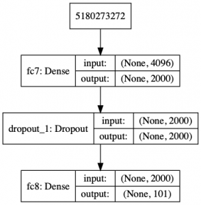
And the results obtained with the various algorithms are:
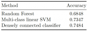 We note that we can’t achieve good performances with Random Forest. Even if this algorithm is fast and simple, it is generally not the best at handling the big amount of features and data sparsity.
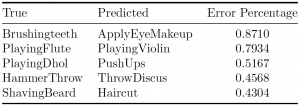
For this task, SVM and neural network are performing better, but they are more computationally expensive.. We want to know which labels are the most common to misclassify according to the neural network. In the next table we report the couple of true and predicted labels for which error rates are the largest.
Further improvements are possible. With more computational power and data, it would be possible to make all (or part of the) weights in the neural network trainable, including the convolutional base parameters, obtaining hopefully better results in the task at hand (i.e. UCF).